
Thermal Demagnetization in NdFeB: Permeance Coefficient (Pc), Load Lines, and Irreversible Loss Prevention
Prevent NdFeB thermal demagnetization: understand permeance coefficient (Pc), read load lines, and use an RFQ checklist to request a magnet grade review.
Published and editorially reviewed: October 26, 2026. Written for global OEM engineers, procurement teams, and incoming quality inspectors selecting sintered NdFeB magnets.
Thermal demagnetization in NdFeB cannot be prevented by a grade suffix alone. Check the magnet's permeance coefficient (Pc), its temperature-dependent demagnetization curves, and the worst opposing field. A catalog temperature is a screening value, not approval for every geometry or magnetic circuit.
For example, selecting N45SH because a catalog lists 150°C does not establish a margin at 125°C ambient: the magnet itself may be hotter, and a thin open-circuit part or motor fault current can create a less favorable operating point. This is an illustrative design scenario, not a reported customer failure or measured loss percentage.
This guide explains the load-line calculation, separates recoverable magnetic loss from material damage, and turns that distinction into a drawing and RFQ checklist. For project-specific inputs, request a magnet grade review.
Scope, Assumptions, and Use Case Boundaries
- Material: Sintered NdFeB, with magnetization along the specified drawing axis. Bonded NdFeB and SmCo require their own material curves.
- Temperature: The selected supplier grade's documented range, below its Curie temperature. No universal operating temperature or fixed temperature derating is assumed.
- Circuits: Open-circuit parts and assemblies with a steel return path. The analytical example below assumes a uniform magnet, a linear recoil segment, and no external opposing field.
- Limits: Edge demagnetization, steel saturation, leakage, rotor heating, and transient or cross-axis fields require appropriate electromagnetic/thermal modeling and representative testing. This guide does not qualify a safety-critical assembly.
- Evidence: Catalog data are identified as supplier examples. Calculations are reproducible screening examples, not Ganzhou Magnets laboratory results, customer case studies, or guaranteed performance.
1. The Three Mechanisms of Magnetic Loss: Clarifying the Physics
When evaluating a failed thermal test, measure again at the original reference temperature before deciding which loss mechanism occurred.
1. Reversible Magnetic Loss
Magnetic output falls as temperature rises and recovers on cooling if no irreversible change has occurred. Temperature coefficients are grade- and interval-specific. For example, Arnold's catalog specifies the measurement interval alongside its coefficients; do not extrapolate a room-temperature coefficient through the knee or across the full operating range.
2. Irreversible Magnetic Loss (Operating Past the Knee)
Elevated temperature reduces resistance to an opposing field. If the local operating state enters the nonlinear demagnetization region, some domains reverse and magnetic output can remain lower after cooling. The loss depends on the material curve, geometry, field distribution, and exposure; Pc alone cannot supply a loss percentage.
Remagnetization may restore magnetic output if the alloy is undamaged. The required saturating field and fixture depend on the grade and assembly. There is no universal “three times Hcj” recovery rule, and assembled parts may need disassembly or replacement.
3. Material Damage and the Curie Distinction
Corrosion, oxidation, and excessive heat can damage the alloy or coating; a magnetic pulse cannot repair consumed or degraded material. Crossing the Curie temperature removes ferromagnetic order while hot, but does not by itself prove permanent lattice destruction. On cooling, magnetic order returns; remagnetization may be possible if no chemical or microstructural damage occurred. Neither cooling nor remagnetization establishes that an overheated assembly is fit for reuse.
Magnetic Loss Mechanism Comparison Matrix
| Mechanism | What changes? | Recovers on cooling? | Can remagnetization help? | Procurement / quality action |
|---|---|---|---|---|
| Reversible loss | Temperature-dependent magnetic output | Yes, if no other loss occurred | Usually unnecessary | Check required hot torque, field, or holding force. |
| Irreversible domain reversal | Magnetization state after knee-region exposure | No | Potentially, if material is undamaged | Review hot curves and worst opposing field. |
| Curie-temperature excursion | Ferromagnetic order disappears while hot | Original magnetization is not assured | Potentially, if material remains intact | Inspect and requalify; do not classify all such events as lattice destruction. |
| Corrosion / metallurgical damage | Material integrity | No | Cannot repair damaged material | Review coating, environment, and thermal exposure. |
2. Demystifying the Permeance Coefficient (Pc) and the Load Line
What is the Permeance Coefficient?
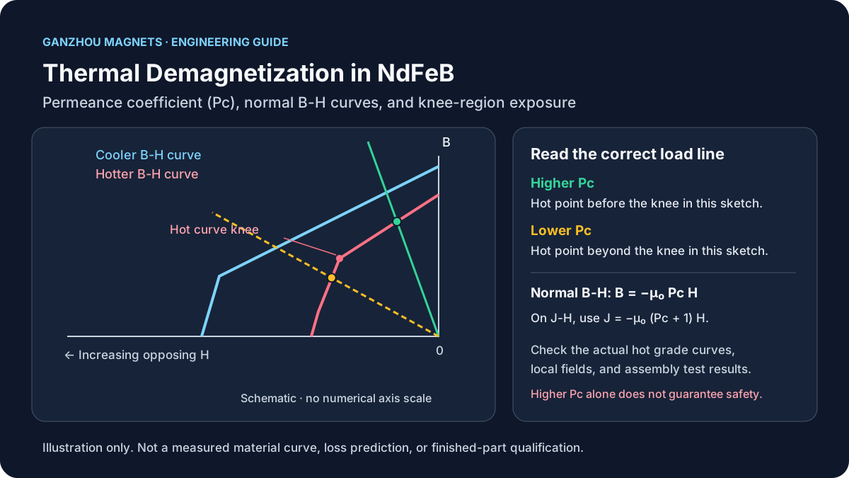
Pc describes the normal B-H load line at a magnet's operating point. Use a positive magnitude for the opposing field Hd; signed H is negative in the second quadrant:
Pc = Bd / (μ0 |Hd|)          SI: B in T, H in A/m
Pc = Bd [gauss] / |Hd| [Oe]  conventional CGS numerical ratio
B = -μ0 Pc H                B-H load line without an applied opposing field
μ0 = 4π × 10⁻⁷ H/m
Do not divide tesla by kA/m without the unit conversion and μ0. The load-line intersection with the normal B-H curve gives the operating B and H. The intrinsic curve uses polarization J = B − μ0H. Therefore the same circuit becomes J = −μ0(Pc + 1)H on a J-H plot; drawing the unmodified B-H load line on J-H gives the wrong operating point.
Conceptual diagram only: curves and slopes are not measured grade data. Higher Pc can improve the operating point, but does not guarantee zero loss. Actual supplier curves are available in the NdFeB catalog.
Why Geometry Matters
Thin magnets along the magnetization axis generally have a less favorable open-circuit operating point than elongated magnets of the same material. Shape, magnetization direction, neighboring magnets, and the return path all matter. A single length-to-diameter expression is not a universal Pc formula for cylinders, blocks, and rings. Use a documented shape-specific demagnetizing-factor model or field simulation, and identify whether its result is local, central, or volume-averaged.
For an ideal uniformly magnetized ellipsoid with SI demagnetizing factor N along the magnetization axis, H = −NM and B = μ0(H + M), giving Pc = (1 − N)/N. This identity does not make an ellipsoid model exact for a disc, rectangular block, or hollow ring.
3. A Reproducible Load-Line Screening Calculation
For an ideal magnetic circuit with one air gap, negligible steel reluctance and leakage, equal magnet/gap flux, and no applied opposing field, Ampère's law and flux continuity give:
|Hm| Lm = Hg Lg
Bm Am = Bg Ag
Bg = μ0 Hg
Pc = (Lm / Lg) × (Ag / Am)
Lm is the magnet length along magnetization; Lg is the total series air-gap length; Am and Ag are the respective cross-sectional areas. Length units must match, as must area units. Leakage, fringing, and steel saturation require a more complete circuit model; the expression is not a motor fault-current calculation.
Illustrative inputs: Lm = 3 mm, Lg = 1 mm, Am = Ag = 100 mm². The ideal circuit gives Pc = 3. On a linear recoil segment, assume Br = 1.20 T and relative recoil permeability μrec = 1.05:
B = Br + μ0 μrec H
B = Br Pc / (Pc + μrec) = 1.20 × 3 / 4.05 = 0.889 T
H = -Br / [μ0 (Pc + μrec)] ≈ -236 kA/m
Doubling the gap to 2 mm gives Pc = 1.5, B = 0.706 T, and H ≈ −374 kA/m. The larger opposing field explains why geometry affects risk. Neither result establishes thermal safety: Br and μrec here are illustrative constants, and both points still need comparison with the selected grade's hot curves. The linear model ceases to predict the operating state correctly beyond the knee.
Six Conditions to Resolve Before Grade Approval
| Design condition | What changes the load line or loss risk? | Required evidence | Buying decision |
|---|---|---|---|
| Thin axial disc | Nonuniform self-demagnetizing field | Shape-specific model and hot curves | Do not approve from diameter and suffix alone. |
| Rectangular plate | Thickness axis and edge fields | Magnetization drawing and local field map | Review thickness before increasing coercivity. |
| Axial ring | Inner and outer edges affect the field | Ring-specific model | Do not substitute an equal-area solid disc without validation. |
| Steel-backed holder | Return-path reluctance and saturation | Steel grade, section, and working gap | Qualify the complete assembly and gap. |
| Motor rotor | Temperature plus armature reaction | Hot local-field analysis at peak/fault current | A nominal Pc does not approve the motor. |
| Oven / incoming inspection | Fixture, soak, and reference measurement | Agreed exposure and post-cooling measurement | Match the test to the purchase specification. |
4. NdFeB Temperature Suffix Grades: Comparing Nominal vs. Low-Pc Realities
Suffixes describe coercivity families, but the exact grade and supplier datasheet control. The examples below come from Arnold's published grade table; they are not Ganzhou Magnets product guarantees or universal suffix minima.
| Supplier example grade | Minimum Hcj (kA/m) | Catalog maximum use temperature | What must still be checked? |
|---|---|---|---|
| N35 | 955 | 80°C | Hot curve and circuit operating point |
| N35M | 1114 | 100°C | Same, including magnet temperature |
| N35H | 1353 | 120°C | Same, including opposing field |
| N35SH | 1592 | 150°C | Same, including local edge fields |
| N35UH | 1990 | 180°C | Same, including thermal duty |
| N35EH | 2388 | 200°C | Same, including coating and retention |
| N35AH | 2706 | 220°C | Same, with assembly qualification |
Do not subtract a fixed number of degrees for “low Pc.” Neither a universal Pc threshold nor a generic temperature penalty can replace the actual temperature curves. Coating, adhesive, and mechanical retention may impose lower limits than the magnetic material. See the NdFeB grade selection page for related sourcing questions.
5. The Cost Optimization Dilemma: Geometry vs. Heavy Rare Earths
Compare a geometry change, a higher-coercivity grade, and a grain-boundary-diffused (GBD) option against the same hot output and irreversible-loss requirement. Increasing thickness may improve the operating point, but reducing pole area to preserve volume can also alter the useful flux, force, or torque. It does not guarantee a particular Pc increase or unchanged cost.
GBD can improve coercivity while limiting heavy rare earth use and remanence penalties, subject to geometry and processing constraints. Ask for a finished-part curve and quote; a suffix does not establish alloy composition or a universal price multiplier. No 2026 commodity price averages or supplier cost surcharges are assumed here.
For an RFQ, send the six-point checklist below with your drawing via Ganzhou Magnets contact, and request comparable evidence for each option before approving a substitution.
6. How to Read a Supplier B-H Curve at Temperature
Ask for both normal B-H and intrinsic J-H curves at the maximum magnet temperature, together with the grade, revision, measurement conditions, and whether curves are typical or guaranteed.
- Read the axes and units. Distinguish B from J, and Hcb (B = 0) from Hcj (J = 0).
- Use the correct load line. Find the B-H intersection, or transform the line correctly for J-H as described in section 2.
- Define the knee criterion. Hk may denote a specified polarization reduction, such as J falling to 90% of Br. Confirm the supplier's definition; it is not an automatic 10% permissible assembly loss.
- Apply worst-case conditions. Include opposing fields, tolerances, and local hot spots. An applied field generally offsets the circuit relation; it is not always another line through the origin.
- Validate the assembly. Use representative thermal/field exposure followed by measurement at the same reference temperature. A room-temperature Hcj certificate alone does not approve hot performance.
7. The Procurement & Drawing Audit Checklist
Before freezing the drawing, engineering, procurement, and quality should agree on:
- 1. Circuit and magnetization: Dimensions, tolerances, magnetization axis, working gaps, steel return path, and the Pc estimation method with its limitations.
- 2. Thermal duty: Maximum magnet temperature, duration, cycles, and heating/cooling conditions; ambient temperature alone is insufficient.
- 3. Opposing fields: Worst running, stall, and fault conditions, plus any assembly or shipping fixtures that alter the magnetic circuit.
- 4. Acceptance measurement: Baseline and post-cooling quantity (magnetic moment, flux in a defined fixture, or application output), reference temperature, instrument, orientation, sampling, and measurement uncertainty.
- 5. Loss limit and exposure: An agreed numerical loss limit with a defined soak and circuit. Example only: “No more than 2.0% loss in magnetic moment after 2 hours at 120°C, open circuit, measured before and after at 20°C in the same calibrated setup.” This is a buyer-defined example, not a universal IEC test or tolerance.
- 6. Comparable supplier options: Hot curves, finished-part qualification, and quotes for geometry, grade, or GBD alternatives; keep the same output requirement when comparing costs.
8. Frequently Asked Questions (FAQ)
Q1: Can irreversible thermal demagnetization be reversed by cooling the magnet down?
No. Reversible temperature loss recovers on cooling; irreversible domain reversal leaves a lower magnetic output at the original reference temperature. A suitable magnetizer may restore an undamaged magnet, but the field and fixture must be qualified for that grade and assembly.
Q2: What is the difference between the B-H curve and the J-H curve?
B-H shows total flux density; J-H shows intrinsic polarization, with J = B − μ0H. A normal load line has B = −μ0PcH. The corresponding intrinsic line has J = −μ0(Pc + 1)H. Use the appropriate line and temperature curve when checking knee-region exposure.
Q3: Why can thin disc magnets demagnetize at lower temperatures than thicker magnets of the same grade?
Their open-circuit geometry generally creates a stronger self-demagnetizing field. The actual limit depends on the grade, magnetization direction, neighboring materials, and external fields. Neither thinness nor Pc alone determines a safe temperature or loss percentage.
Q4: How can incoming quality control test irreversible thermal loss?
Use an agreed, calibrated measurement of magnetic moment or flux in a defined fixture. A Helmholtz-coil/fluxmeter setup may measure magnetic moment when appropriately calibrated; do not label every coil reading as total open-circuit flux. Record Q1 at the reference temperature, expose the part to the agreed thermal/field cycle, cool to the same reference temperature, and record Q2 in the same orientation and fixture:
Irreversible loss (%) = 100 × (Q1 − Q2) / Q1For illustrative readings Q1 = 1.000 and Q2 = 0.985 in the same units, the calculated loss is 1.5%. These are example inputs, not test results. Define the allowable limit, exposure, sample plan, and uncertainty in the purchase specification.
Q5: When should an engineer compare NdFeB with samarium-cobalt?
Compare SmCo when the required temperature stability or hot magnetic output is difficult to achieve with NdFeB. Check the actual temperature curves, corrosion environment, mechanical constraints, and total assembly cost. There is no single temperature at which every application should switch materials.
Request a Load-Line and Magnet Grade Review
Send Ganzhou Magnets your drawing, magnetization axis, working gap, maximum magnet temperature, opposing-field conditions, target quantity, and allowable post-cooling loss. Ask for the proposed grade, available hot curves, and a qualification plan before releasing the purchase order.
Sources & Reference Limits
- Arnold Magnetic Technologies — Neodymium Iron Boron Magnets. Source for the specific supplier-grade examples and GBD overview. Supplier catalog maxima do not establish installed performance.
- Arnold Magnetic Technologies — Neodymium Iron Boron Magnet Catalog. Includes temperature-dependent B-H/J-H curves, Pc lines, and coefficient measurement intervals; the N42SH sheet is printed page 34 (PDF page 34). Use the required grade's current revision for approval.
- Arnold Magnetic Technologies — Grain Boundary Diffused Neo Catalog. Additional supplier reference for GBD options, linked from the official product page. This PDF was not independently fetched in this review; request the applicable revision with the quote.
Review limits: Product page and main catalog reviewed October 26, 2026. These three URLs are from one manufacturer, not independent corroborating studies. Equations above are derived from the stated ideal-circuit assumptions; neither catalog curves nor illustrative arithmetic constitute finished-part test evidence. The sampling plan, exposure, and loss limit require buyer/supplier agreement. Recheck the applicable datasheet before design release and after any grade, geometry, or duty change; the next editorial review is due by October 2027.
Categories
More Posts

Rare Earth Permanent Magnets Market Update (2026-W16): Buyer Hold Points Before Q2 Disclosures
April 2026 buyer update on NdFeB and Sm: verified 30-day changes, unresolved risks, and sourcing actions for US, EU, and LATAM teams before Q2 disclosures.


Rare Earth Permanent Magnets Market Update (2026-W18): Derivative Tariff Corrections Add a New Compliance Gate
Week 18 rare earth magnets update: U.S. derivative-duty corrections, NdFeB and Sm supply signals, and immediate sourcing actions for US, EU, and LATAM buyers.

NdFeB vs SmCo: Guía completa de comparación de imanes para ingenieros
Comparación detallada de imanes de neodimio (NdFeB) y samario-cobalto (SmCo) que cubre rendimiento magnético, estabilidad térmica, resistencia a la corrosión, costo y recomendaciones por aplicación.